Building a HazImp job

Templates

The simplest way to use HazImp is with a template, which sets up a PipeLine to run a collection of Job functions. There are currently templates for wind, earthquake and flood hazard events. Templates take into account internal vulnerability curves and the data flow needed to produce loss information, simplifying the configuration file.

Templates are used to set out the flow of processing invoked in separate Job functions that are then connected into a PipeLine that is subsequently executed.

Note

Because some of the Job functions in the templates are essential, the order of key/value pairs in the configuration files is important. The code will raise a RuntimeError if the order is incorrect, or if a mandatory configuration key is missing. This is even more important if not using the pre-defined templates.

We take the example of the wind_v4 template. It sets up the following job sequence in a specific order:

1. LOADCVSEXPOSURE - load the exposure data

2. LOADRASTER - load the hazard raster data

3. LOADXMLVULNERABILITY - load the vulnerability functions

4. SIMPLELINKER - select a group of vulnerability functions - some vulnerability files may have multiple sets of curves identified by vulnerabilitySetID

5. SELECTVULNFUNCTION - link the selected vulnerability function set (specified by the vulnerabilitySetID option) to each exposure asset

6. LOOKUP - do a table lookup to determine the damage index for each asset, based on the intensity measure level (e.g. the wind speed)

7. CALCSTRUCTLOSS - combine the calculated damage index with the building value to calculate $$$ loss

8. SAVE - should speak for itself - saves the building level loss data

9. SAVEPROVENANCE - saves provenance data (like the version of HazImp, source of the hazard data, etc.)

Available templates

There are currently 6 templates pre-packaged with HazImp (plus one deprecated template). Most are built around wind impacts, but there are also templates for earthquake and flood (both structural and contents losses):

1. ‘wind_v3’ - (DEPRECATED) a basic wind impact template for structural loss and structural loss ratio.

2. ‘wind_v4’ - Base wind impact template. Allows user to specify the vulnerability function set in the configuration.

3. ‘wind_v5’ - Optional categorisation and tabulation of output data.

4. ‘wind_nc’ - Includes option to permute exposure data for mean and upper limit of impact (structural loss ratio).

5. ‘earthquake_v1’ - Base earthquake impact template. Allows similar functions (aggregation, permutation, etc.) to the wind_nc template.

6. ‘flood_fabric_v2’ - calculate structural loss due to flood inundation.

7. ‘flood_contents_v2’ - contents loss due to flood inundation.

Saving to geospatial formats

Data can optionally be saved to a geospatial format that aggregates the impact data to spatial regions (for example suburbs, post codes).

aggregate

This will activate the option to save to a geospatial format.

boundaries

The path to a geospatial file that contains polygon features to aggregate by

filename

The path to the output geospatial file. This can be either an ESRI shape file (extension shp), a GeoJSON file (json) or a GeoPackage (gpkg). If an ESRI shape file is specified, the attribute names are modified to ensure they are not truncated. Multiple filenames can be specified in a list format.

impactcode

The attribute in the exposure file that contains a unique code for each geographic region to aggregate by.

boundarycode

The attribute in the boundaries file that contains the same unique code for each geographic region. Preferably the impactcode and boundarycode will be of the same type (e.g. int or str)

categories

If True, and the Categorise job is included in the pipeline, the number of assets in each damage state defined by the categories will be added as an attribute to the output file for each geographic region. Note the different spelling used in this section.

Presently, HazImp will aggregate the following fields:

'structural': 'mean', 'min', 'max'
'contents': 'mean', 'min', 'max'

If permutation of the exposure is performed, then the corresponding ‘_max’ field can also be included in the aggregation:

'structural_max': 'mean', 'min', 'max'

Example:

- aggregate:
    boundaries: QLD_Mesh_Block_2016.shp
    filename: QLD_MeshblockImpacts.shp
    impactcode: MB_CODE
    boundarycode: MB_CODE16
    categories: True
    fields:
     structural: [ mean ]

Output data to multiple files:

- aggregate:
  boundaries: northwestcape_meshblocks.geojson
  boundarycode: MB_CODE11
  impactcode: MESHBLOCK_CODE_2011
  filename: [olwyn_impact.shp, olwyn_impact.json]
  categories: True
  fields:
     structural: [mean]

Note

The length of some attribute names exceeds the maximum length allowed for ESRI shape files and will be automatically truncated when saving to that format. A warning message will be generated indicating this truncation is being applied.

Aggregate with permuted exposure:

- aggregate:
  boundaries: northwestcape_meshblocks.geojson
  boundarycode: MB_CODE11
  impactcode: MESHBLOCK_CODE_2011
  filename: [olwyn_impact.json]
  categories: True
  fields:
     structural: [mean]
     structural_max: [mean]

This option has only been implemented in the wind_nc and wind_v5 templates at this time (June 2021).

Including categorisations

Users may want to convert from numerical values to categorical values for output fields. For example, converting the structural loss ratio from a value between 0 and 1 into categories which are descriptive (see the table below).

Lower value	Uppper value	Category
0	0.02	Negligible
0.02	0.1	Slight
0.1	0.2	Moderate
0.2	0.5	Extensive
0.5	1.0	Complete

The Categorise job enables users to automatically perform this categorisation. Add the “categorise” section to the configuration file to run this job. This is based on the pandas.cut method.

categorise

This will enable the Categorise job. The job requires the following options to be set.

field_name

The name of the created (categorical) field in the context.exposure_att DataFrame

bins

Monotonically increasing array of bin edges, including the rightmost edge, allowing for non-uniform bin widths. There must be (number of labels) + 1 values, and range from 0.0 to 1.0.

labels

Specifies the labels for the returned bins. Must be the same length as the resulting bins.

Example

A basic example, which would result in the categories listed in the table above being added to the column “Damage state”:

- categorise:
   field_name: 'Damage state'
   bins: [0.0, 0.02, 0.1, 0.2, 0.5, 1.0]
   labels: ['Negligible', 'Slight', 'Moderate', 'Extensive', 'Complete']

Another example with three categories. See the example configuration in examples/wind/three_category_example.yaml

- categorise:
   field_name: 'Damage state'
   bins: [0.0, 0.1, 0.5, 1.0]
   labels: ['Minor', 'Moderate', 'Major']

See also the Saving to geospatial formats documentation to categorise spatial aggregations using these configurations.

Generate tables

A common way of reporting the outcomes of a HazImp analysis is to look at the number of features distributed across various ranges. For example, the number of buildings in a given damage state, grouped by an age category. While many may want to do their own pivot tables on the output, this can automate the process for the most common index/column combination.

Construction era	Negligible	Slight	Moderate	Extensive	Complete
1914 - 1946	9542	311	25	46	7
1947 - 1961	10496	113	11	1	0
1962 - 1981	23984	909	73	57	8
1982 - 1996	25676	914	186	39	1
1997 - present	16675	711	115	40	3

The Tabulate job performs a pivot table operation on the context.exposure_att DataFrame and writes the results to an Excel file. Add the “tabulate” section to the configuration file to run this job. This is closely based on pandas.DataFrame.pivot_table.

tabulate

Run a tabulation job

file_name

Destination for the output of the tabulation. Should be an Excel file

index

Keys to group by on the pivot table index. If a list is passed, it is used as the same manner as column values.

columns

Keys to group by on the pivot table column. If a list is passed, it is used as the same manner as column values.

aggfunc

function, list of functions, dict, default numpy.mean If a list of functions passed, the resulting pivot table will have hierarchical columns whose top level are the function names (inferred from the function objects themselves) If dict is passed, the key is column to aggregate and value is function or list of functions.

Examples

- tabulate:
   file_name: wind_impact_by_age.xlsx
   index: YEAR_BUILT
   columns: Damage state
   aggfunc: size

This will return a table of the number (the size function) of buildings in each damage state, grouped by the “YEAR_BUILT” attribute, and saved to the file “wind_impact_by_age.xlsx”

- tabulate:
   file_name: mean_slr_by_age.xlsx
   index: YEAR_BUILT
   columns: structural_loss_ratio
   aggfunc: mean

This will return a table of the mean structural loss ratio of buildings, grouped by the “YEAR_BUILT” attribute, and saved to the file “mean_slr_by_age.xlsx”

Using permutation to understand uncertainty in vulnerability

In many regions (in Australia), the attributes of individual buildings are unknown, but are recorded for some statistical area (e.g. suburb, local government area). In this case, the vulnerability curve assigned to a building may not be precisely determined, which can lead to uncertainty in the impact for a region.

To overcome this, users can run the impact calculation multiple times, while permuting the vulnerability curves for each region (suburb, local government area, etc.). This requires some additional entries in the template file.

exposure_permutation

This section describes the Exposure data attribute that will constrain the permutation, and the number of permuations.

groupby The field name in the Exposure data data by which the assets will be grouped. While any categorical attribute could be used (e.g. building age), it is recommended to use an attribute that represents the geographical region.

iterations The number of iterations to perform. Default is 1000 iterations

quantile The quantile to represent the range of outcomes. Default=[0.05, 0.95] (5th and 95th percentile)

Example:

- exposure_permutation:
    groupby: MB_CODE
    iterations: 1000

The resulting output calculates a mean loss per building from all permutations,

as well as lower and upper loss estimats, which is the permutation that provides the lowest and highest mean loss over all buildings. In reality, we actually use the 5th and 95th percentile of the mean loss to determine these extremes of the distribution. The values are stored in an attribute with the suffix ‘_lower’ and ‘_upper’ appended.

An example of aggregation to geospatial fomats using permutation is given in the Saving to geospatial formats section.

As a demonstration, the figure below shows three permutations of the location of different asset types within a geographic region. The hazard intensity level is shown by the blue to red shading. In each permutation, the different assets are in different locations. The total number of each type of asset remains the same within the region. Therefore, depending on the permutation, the hazard levels that building types are exposed to varies. This is reflected in the resulting damage index values for the region, shown below.

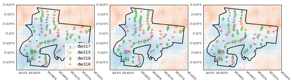
Fig. 3 Demonstration of permutation of exposure. In each panel, the number of each asset type is the same, but they are randomly assigned to the asset locations.

In each permutation, the hazard intensity sampled by the assets of one type will vary, leading to different levels of loss among those assets. This results in a different distribution of losses across the region. Below is the distribution of structural loss ratio for each iteration across the region.

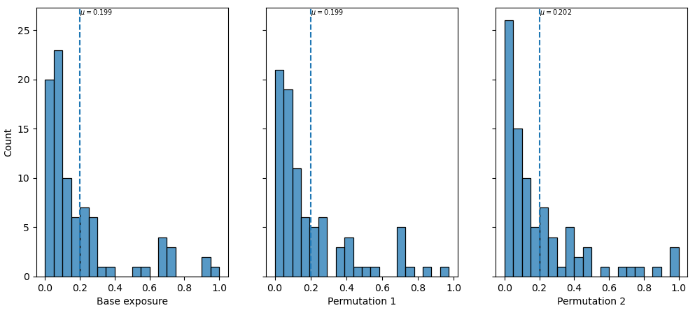
Fig. 4 Distribution of structural loss ratio across the geographic region. The vertical line indicates the mean loss ration in the region. Note the value changes slightly between iterations.

If there is greater variability in the hazard across the region, we are likely to see greater variability in the resulting distribution. In contrast, if the hazard level is uniform across the region, then there will be little to no variability in the permutations. Similarly a more diverse range of asset types (specifically with a wide range of vulnerabilities) will lead to greater variability as well, when there’s at least moderate variability in the hazard level.