Using permutation to understand uncertainty in vulnerability

In many regions (in Australia), the attributes of individual buildings are unknown, but are recorded for some statistical area (e.g. suburb, local government area). In this case, the vulnerability curve assigned to a building may not be precisely determined, which can lead to uncertainty in the impact for a region.

To overcome this, users can run the impact calculation multiple times, while permuting the vulnerability curves for each region (suburb, local government area, etc.). This requires some additional entries in the template file.

exposure_permutation

This section describes the Exposure data attribute that will constrain the permutation, and the number of permuations.

groupby The field name in the Exposure data data by which the assets will be grouped. While any categorical attribute could be used (e.g. building age), it is recommended to use an attribute that represents the geographical region.

iterations The number of iterations to perform. Default is 1000 iterations

quantile The quantile to represent the range of outcomes. Default=[0.05, 0.95] (5th and 95th percentile)

Example:

- exposure_permutation:
    groupby: MB_CODE
    iterations: 1000

The resulting output calculates a mean loss per building from all permutations,

as well as lower and upper loss estimats, which is the permutation that provides the lowest and highest mean loss over all buildings. In reality, we actually use the 5th and 95th percentile of the mean loss to determine these extremes of the distribution. The values are stored in an attribute with the suffix ‘_lower’ and ‘_upper’ appended.

An example of aggregation to geospatial fomats using permutation is given in the Saving to geospatial formats section.

As a demonstration, the figure below shows three permutations of the location of different asset types within a geographic region. The hazard intensity level is shown by the blue to red shading. In each permutation, the different assets are in different locations. The total number of each type of asset remains the same within the region. Therefore, depending on the permutation, the hazard levels that building types are exposed to varies. This is reflected in the resulting damage index values for the region, shown below.

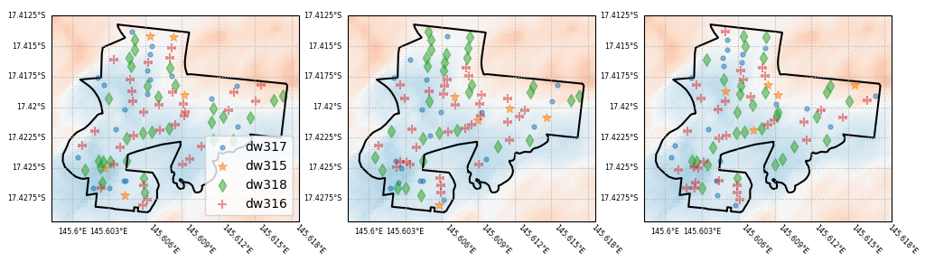
Demonstration of permutation of exposure. In each panel, the number of each asset type is the same, but they are randomly assigned to the asset locations.

In each permutation, the hazard intensity sampled by the assets of one type will vary, leading to different levels of loss among those assets. This results in a different distribution of losses across the region. Below is the distribution of structural loss ratio for each iteration across the region.

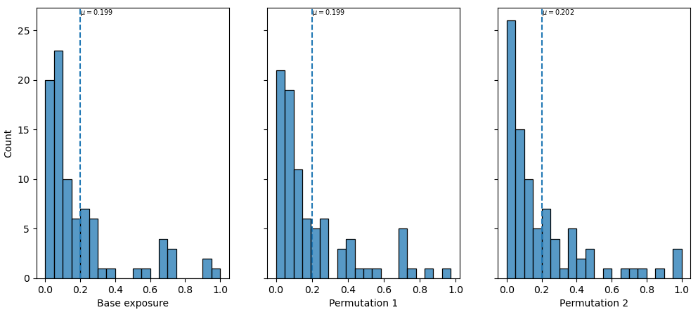
Distribution of structural loss ratio across the geographic region. The vertical line indicates the mean loss ration in the region. Note the value changes slightly between iterations.

If there is greater variability in the hazard across the region, we are likely to see greater variability in the resulting distribution. In contrast, if the hazard level is uniform across the region, then there will be little to no variability in the permutations. Similarly a more diverse range of asset types (specifically with a wide range of vulnerabilities) will lead to greater variability as well, when there’s at least moderate variability in the hazard level.